This article introduces how to conduct feature engineering for model training and prediction in DolphinDB. Inspired by the 1st place solution of the time series prediction competition Kaggle Optiver Realized Volatility Prediction, we propose a solution applicable to both batch and stream processing in DolphinDB to fit in comprehensive machine learning application scenarios. The comparison shows that DolphinDB delivers about 30x performance improvement than Python pandas.

The examples in this tutorial use DolphinDB server (Enterprise Edition) 2.00.6 and above.

1. Snapshot Market Data

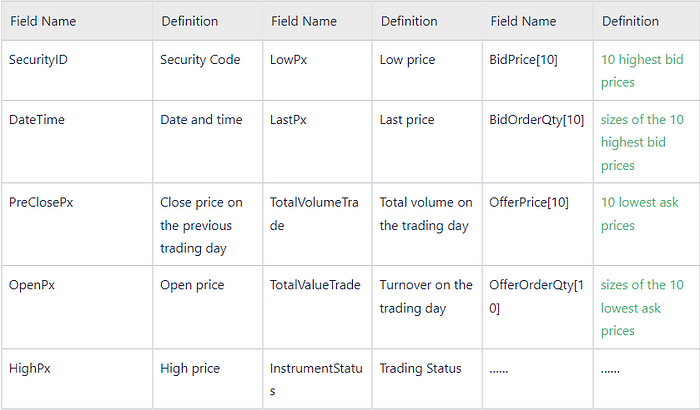
The data used in this project is 3-second snapshots of level 2 tick data. It contains the following columns:

2. Feature Engineering

2.1 Technical Indicators

The following indicators are calculated based on the 10 highest bid prices and 10 lowest ask prices mentioned above.

wap: weighted average price

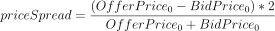
priceSpread: bid-ask spread

bidSpread: difference between the lowest and second lowest bid prices

offerSpread: difference between the highest and second highest ask prices

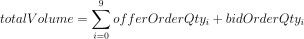
totalVolume: total size of the 10 highest bids and 10 lowest asks

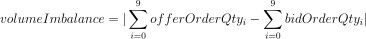
volumeImbalance: absolute value of the difference between the sizes of 10 highest bid prices and 10 lowest ask prices

logReturnOffer: log return of ask price

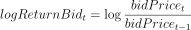
logReturnBid: log return of bid price

wapBalance: absolute value of wap difference

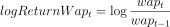
logReturnWap: log return of wap

2.2 Derived Features

The derived features are generated by aggregating over the indicators with 10-minute windows.

The following aggregate functions are used:

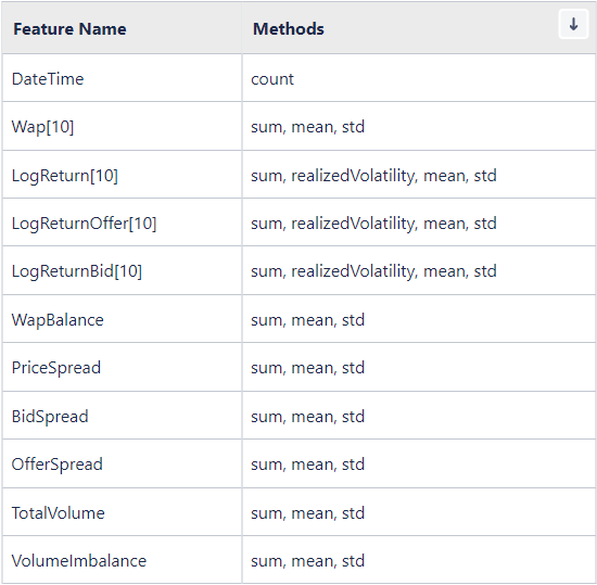
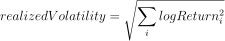
We will predict the realized volatility:

realizedVolatility: realized volatility

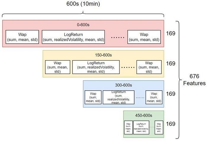
Considering the features are time-sensitive, we form 4 overlapping windows based on the 10-minute window (0–600s, 150–600s, 300–600s, and 450–600s) and conduct calculations on all of them.

Finally, 676 dimensions of derived features are generated.

3. DolphinDB Metaprogramming

This section introduces how to generate features in batches with metaprogramming (see Metaprogramming — DolphinDB 1.3 documentation).

The DolphinDB scripts for batch processing define an aggregate function featureEngineering which calculate the indicators and generate derived features in batches with metaprogramming.

3.1 Calculation of Indicators

The following part in function featureEngineering calculates the indicators:

3.2 Calculation of Derived Features

In Python, we can pass a dictionary (where key is column names and value is a list of aggregate functions) to the pandas function groupby.agg to implement aggregation on selected columns.

In DolphinDB, we use a user-defined function to convert the above dictionary to SQL statements with metaprogramming.

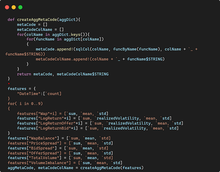
It returns a vector of metacode and the corresponding column names:

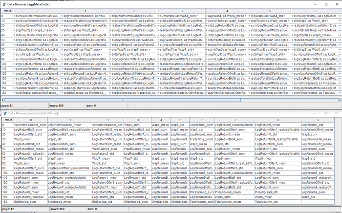
The function featureEngineering generates a table with indicators and renamed columns, which facilitates the calculation of derived features with metaprogramming.

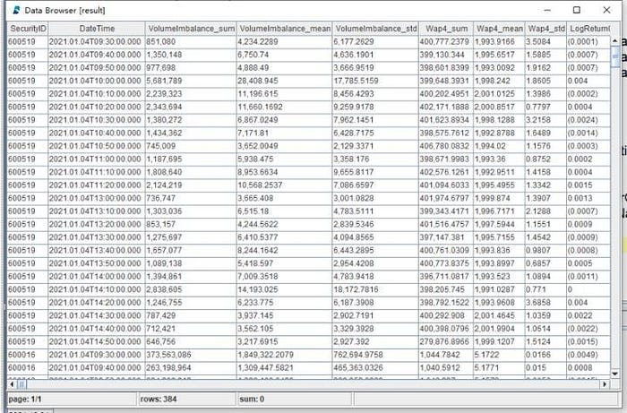
Finally, the metacode is passed to function featureEngineering and the derived features are calculated based on the table generated in the last step. It returns a matrix with 676 columns.

Part of the output table:

See the full scripts of calculating 676 derived features with DolphinDB metaprogramming:

Batch processing in DolphinDB: storing 10 highest bids and 10 lowest asks with multiple columns
Batch processing in DolphinDB (with array vectors): storing 10 levels of quotes with array vectors

4. DolphinDB vs Python

In this article, the performances of Python and DolphinDB regarding feature engineering are compared.

Data: 3-second snapshots of level 2 tick data of 16 securities of a year. The total number of records is 19,220,237.
Calculation: Perform aggregation on each column with 10-minute windows in each group to generate 676 derived features.
Scripts:

Batch processing in DolphinDB: storing 10 levels of quotes with multiple columns

Batch processing in DolphinDB (with array vectors): storing 10 levels of quotes with array vectors

Batch processing in Python

Since DolphinDB adopts distributed parallel computing, the parallelism in the project is configured to 8 (i.e., the tasks are processed by 8 CPU cores simultaneously). For a fair comparison, the Python script also uses 8 processors for parallel processing.

The execution time of the script is 3039 seconds in Python, while in DolphinDB it only takes 100 seconds. The result shows that feature engineering in DolphinDB outperforms Python by around 30 times.

5. Modeling

DolphinDB provides users with many common machine learning algorithms such as least squares regression, random forest, and K-means for regression, classification and clustering, etc.

XGBoost is an optimized distributed gradient boosting library designed to be highly efficient, flexible and portable. XGBoost provides a parallel tree boosting (also known as GBDT, GBM) that solves many data science problems in a fast and accurate way.

In this project, DolphinDB XGBoost plugin is used for model training and prediction.

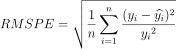
Evaluation Metric: Root Mean Square Percentage Error, RMSPE

See script of Model building and training

5.1 Data Processing

The following script first excludes records with NULL values from the table. The metric LogReturn0_realizedVolatility is used to label the results. The table is adjusted to be passed to the XGBoost method.

Note: This project aims to predict the realized volatility in the next 10 minutes. As Wap_0 is the closest to the stock price, we use LogReturn0_realizedVolatility (which is calculated based on Wap_0) as the label.

5.2 Train Test Split

We do not set validation dataset in this project. The data is split into training set and testing set with a 70–30 split.

5.3 Training and Evaluation

[DolphinDB XGBoost plugin](github.com/dolphindb/DolphinDBPlugin/blob/r..) provides the following 4 methods:

xgboost::train(): train a model
xgboost::predict: make predictions with a model
xgboost::saveModel: save a model to disk
xgboost::loadModel: load a model from disk

The following script is used for model training and evaluation in DolphinDB:

Result:

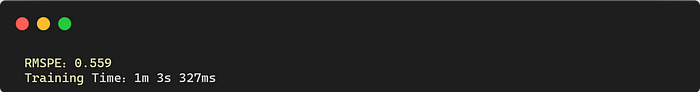
Prediction Performance Evaluation

6. Stream Processing

Calculations in the previous chapters are batch processing of historical data. However, data is often generated as “streams” in production environments, and it is quite challenging to apply the complex computational logic of derived features to stream processing.

To handle such problem, DolphinDB offers various built-in stream engines to provide low-latency solutions.

Stream processing in DolphinDB

Test data (3-second snapshots of level 2 tick data)

6.1 Streaming Framework

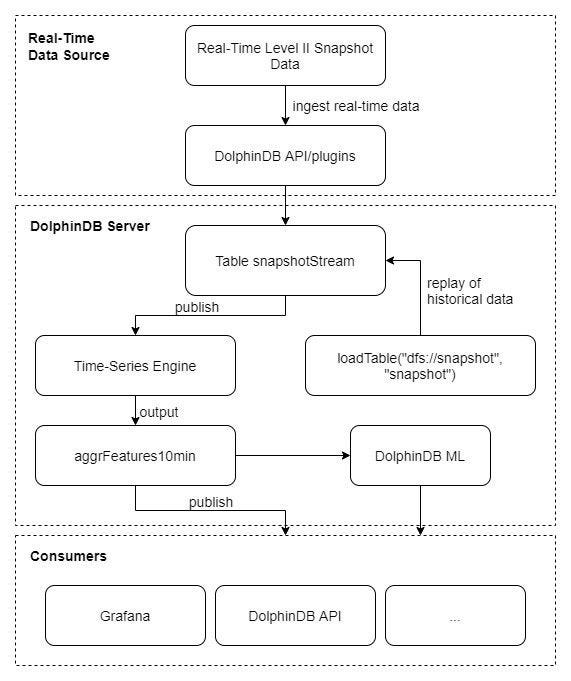
The above diagram depicts the streaming process:

Ingest real-time stream data into table snapshotStream via DolphinDB API;
Subscribe to the table and ingest the data into DolphinDB time-series stream engine where calculations are conducted in a sliding window of 10 minutes (with step of 10 minutes).

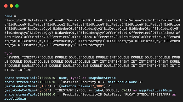
The following is the main script for stream processing:

Create the following stream tables:

snapshotStream: to store the snapshot data

2. aggrFeatures10min: the output table of feature engineering

3. result10min: the output table of predictions

First subscription: subscribe to table snapshotStream

Second subscription: subscribe to table aggrFeatures10min

As DolphinDB has implemented a unified framework of batch and stream processing, the function featureEngineering called in the metrics defined above is identical to the user-defined function featureEngineering used in batch processing.

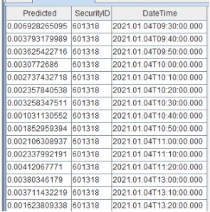
After constructing the streaming framework, the test data is replayed into a shared stream table. The predicted realized volatility is output as follows:

6.2 Latency

In this section, we measure the computational latency in the time-series engine. It consists of 2 parts: the execution time of calculating aggregate features and of predicting realized volatility.

Measure the execution time of calculating aggregate features:

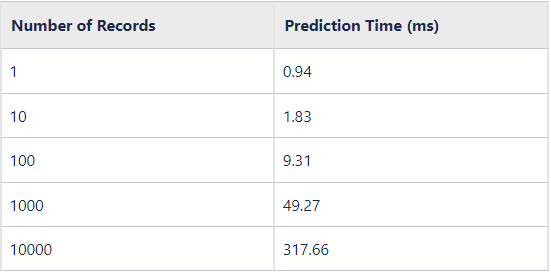
Measure the execution time of predicting realized volatility:

Results

7. Conclusion

This tutorial introduces a unified batch and stream processing solution in DolphinDB for machine learning use cases. Specifically, the same function can be applied to historical data or real-time stream data to generate derived features highly efficiently and conveniently. We construct 10-minute features based on 3-second snapshot data to generate 676 derived features for performance comparison. The comparison shows that our proposed solution is 30 times faster than Python.

Thanks for your reading! To keep up with our latest news, please follow our Twitter @DolphinDB_Inc and Linkedin. You can also join our Slack to chat with the author!

DolphinDB's Blog