Calculating pairwise correlations of securities sheds light on the relationship between different securities, assisting in investment decision-making and risk management. In this article, you’re going to learn how to calculate the pairwise correlations of multiple securities using high frequency data.
The tool we use is DolphinDB and the data we use is the high-frequency quote data of US stocks on August 1, 2007. The raw data is 16.1 GB with 380 million records. We will calculate the pairwise correlations of the most actively traded 500 stocks in that day.
Let’s delve into the code.
select count(*) from loadTable("dfs://TAQ", "quotes") where date= 2007.08.01

def getStockCorrelation(dateValue, num){
    quotes = loadTable("dfs://TAQ", "quotes")

    syms = (exec count(*) from quotes where date = dateValue, time between 09:30:00 : 15:59:59, 0<bid, bid<ofr, ofr<bid*1.1 group by Symbol order by count desc).Symbol[0:num]
    priceMatrix = exec avg(bid + ofr)/2.0 as price from quotes where date = dateValue, Symbol in syms, 0<bid, bid<ofr, ofr<bid*1.1, time between 09:30:00 : 15:59:59 pivot by time.minute() as minute, Symbol
    retMatrix = each(def(x):ratios(x)-1, priceMatrix)
    correlationMatrix = corrMatrix(retMatrix[1:,].ffill())

    mostCorrelated = select * from table(correlationMatrix.columnNames() as sym, correlationMatrix).unpivot(`sym, syms).rename!(`sym`corrSym`corr) context by sym having rank(corr,false) between 1:10
    return mostCorrelated
}

dateValue = 2007.08.01
num = 500
timer mostCorrelated = defStockCorrelation(dateValue,num)
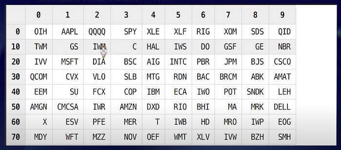
First, we generate a vector of 500 stock tickers with the largest number of quote records.
syms = (exec count(*) from quotes where date = dateValue, time between 09:30:00 : 15:59:59, 0<bid, bid<ofr, ofr<bid*1.1 group by Symbol order by count desc).Symbol[0:num]

Why we use “exec” statement?
The syntax of the “exec” statement is the same as the “select” statement except that “select” always returns a table whereas “exec” can return a scalar, vector, matrix or table, which is more convenient for certain operations.
Next, we select the records for these 500 stocks and filter out dirty data, then generate a minute-level mid-price matrix with stock tickers as column labels and minutes as row labels.
priceMatrix = exec avg(bid + ofr)/2.0 as price from quotes where date = dateValue, Symbol in syms, 0<bid, bid<ofr, ofr<bid*1.1, time between 09:30:00 : 15:59:59 pivot by time.minute() as minute, Symbol

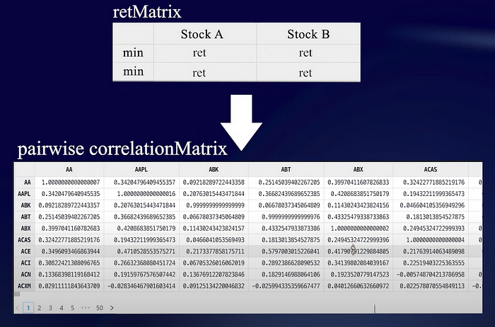
Then convert the minute-level mid-price matrix into a stock return matrix.
retMatrix = each(def(x):ratios(x)-1, priceMatrix)

Based on the stock return matrix, we calculate the correlation between every two columns to get a 500 by 500 pairwise correlation matrix.
correlationMatrix = corrMatrix(retMatrix[1:,].ffill())

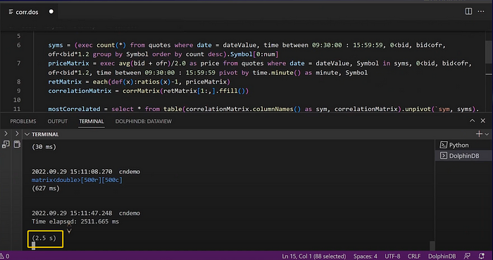
So actually, it only takes 4 lines of code to get the pairwise correlation matrix from the high frequency data in DolphinDB.
In addition, running the script only takes 2.5 seconds.

To verify the accuracy, we get the 3 stocks with the highest correlation with Lehman Brothers from the pairwise correlation matrix. The outputs are Morgan Stanley, Goldman Sachs, and Merrill Lynch, which are all investment bank stocks that are supposed to be highly correlated with Lehman Brothers.
In this example, DolphinDB demonstrates excellent performance in data analysis of large amounts of data with elegant code and minimal coding efforts. The calculation process can be encapsulated into a function to be used in script as well as through various APIs such as Python, C++, Java, C#, Go, etc.
addFunctionView(getStockCorrelation)
Follow the video below to try the efficient calculation!
